Lesson 12: Plot Measurements

This walk-through will demonstrate how to create and evaluate formulaic measurements and noise plots in OrCAD PSpice Designer 22.1. After you complete this topic, you will be able to:

• Create and evaluate measurements
• Use formulas to create a noise plot
• Configure the simulation plot to display previous data

To follow along, continue with the design from the previous topic or use the provided materials.

If materials were not downloaded at the beginning of the walk-through, files for this lesson can be accessed through the materials tab above.

Creating Noise Plots

Step 1: In the schematic page, select PSpice > Edit Simulation Profile from the menu.

Note: If you still have the plots from the last walk-through open, close them.

Step 2: Change the End Frequency to 1G. Click OK.

Step 3: Select PSpice > Run from the menu.

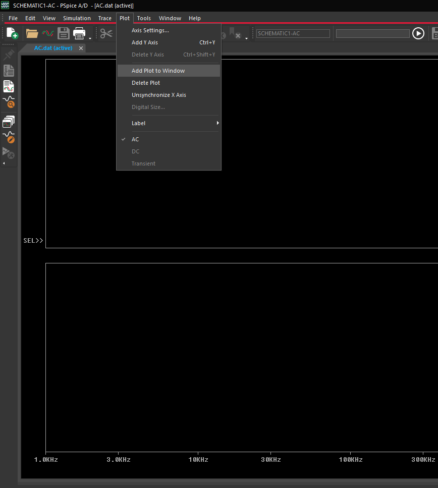
Step 4: In the result window, select Plot > Add Plot to Window from the menu to add a new plot to the window.

Step 5: Select Trace > Add Trace from the menu.

Step 6: Select V(VOUT) from the Simulation Output Variables list. Click OK to add the trace to the upper plot.

Step 7: Select the bottom plot and select Trace > Add Trace again.

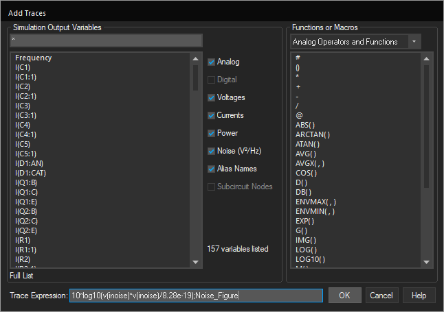
Step 8: Copy the expression 10*log10(v(inoise)*v(inoise)/8.28e-19);Noise_Figure and paste into the Trace Expression field.

Note: This will create a trace with the defined expression and assign the name Noise_Figure.

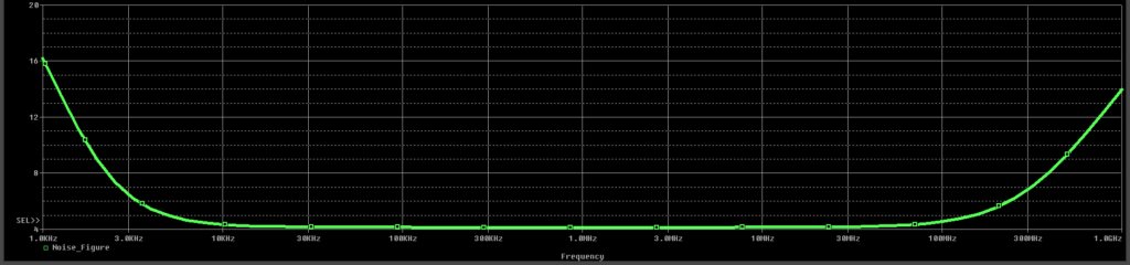
Step 9: Click OK to save the settings. View the plot. Noise_Figure starts at 16 and decreases from there.

Creating Evaluate Measurements

Step 10: Select View > Measurement Results from the menu.

Step 11: Select Trace > Evaluate Measurement.

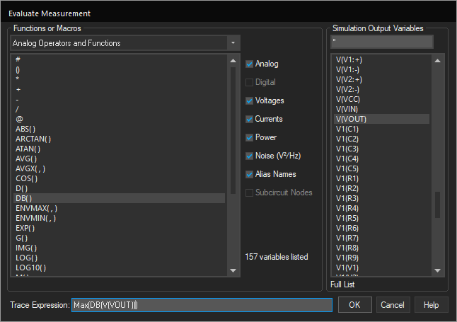
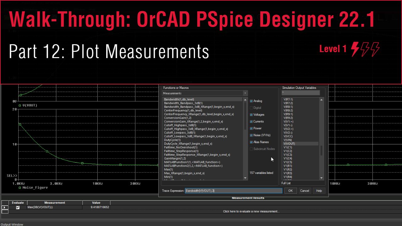
Step 12: The Evaluate Measurement window opens. Select Max(1) from the Functions or Macros list on the left.

Step 13: Select Analog Operators and Functions from the Functions or Macros drop-down menu.

Step 14: Select DB() from the Functions or Macros list.

Step 15: Select V(VOUT) from the Simulation Output Variables list.

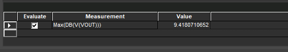
Step 16: Click OK. The measurement is added to the Measurement Results list.

Note: The value of the measurement is automatically calculated and added in the cell to the right of the measurement.

Step 17: Select Click Here to Evaluate a New Measurement.

Step 18: Select Bandwidth(1, db_level) from the Functions or Macros list.

Step 19: Select V(VOUT) from the Simulation Output Variables list.

Step 20: Use your keyboard to enter 3 as the other parameter for a 3dB cutoff.

Step 21: Click OK. The measurement is added to the Measurement Results list.

Step 22: Select Click Here to Evaluate a New Measurement.

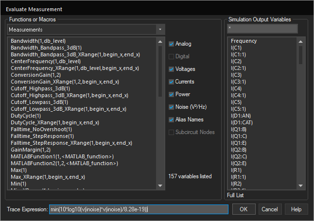
Step 23: Copy the expression min(10*log10(v(inoise)*v(inoise)/8.28e-19)) and use CTRL-V to paste it into the Trace Expression box.

Step 24: Click OK. The measurement is added to the Measurement Results list.

Reusing a Plot Display

Step 25: Select Simulation > Edit Profile from the menu or the Edit Simulation Settings button from the toolbar.

Step 26: Select the Probe Window subpanel from the list on the left side of the window.

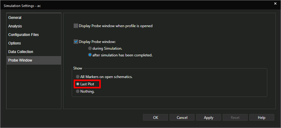
Step 27: Under Show, select Last Plot. Click OK to save the settings and close the window.

Note: This will configure the plot with the same settings, traces, plots, and measurements as the previous simulation. In this example, whenever the plot window is opened it will show the V(VOUT) and Noise_Figure traces.