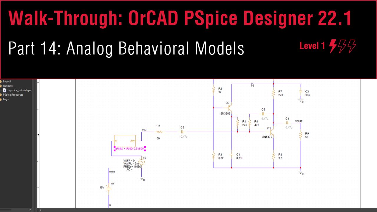
Lesson 14: Analog Behavioral Models

This walk-through will demonstrate how to use analog behavioral models (ABMs) to simulate noise and an ideal low-pass filter in the RF Amplifier circuit in OrCAD PSpice Designer 22.1. After you complete this topic, you will be able to:

• Use an analog behavioral model to define noise and analyze results in the time domain
• Use an analog behavioral model to define a low-pass filter and analyze the results in the frequency domain

To follow along, continue with the design from the previous topic or use the provided materials.

If materials were not downloaded at the beginning of the walk-through, files for this lesson can be accessed through the materials tab above.

Creating a Noise ABM

Step 1: Click and drag to select the sine source, V2, the wire connecting it to ground, and the ground symbol.

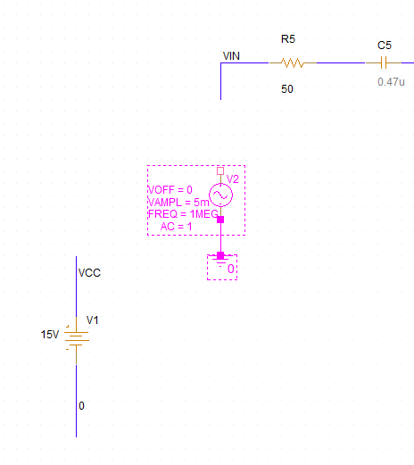
Step 2: Hold Alt on the keyboard and click and drag to move the source further down.

Note: Adjust the position of V1 as needed.

Step 3: Select Place > Component from the menu.

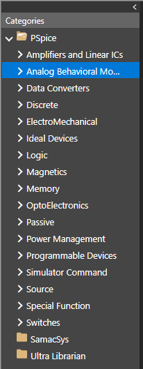
Step 4: Expand the PSpice category and select Analog Behavioral Models.

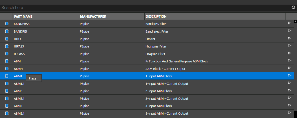
Step 5: Select ABM1 from the list. Right-click and select Place.

Step 6: Click to place the ABM in the schematic. Right-click and select End Mode.

Step 7: Select Place > Wire from the menu, the Wire button from the toolbar, or press W on the keyboard.

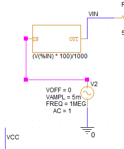
Step 8: Click to add traces between V2, the ABM, and net VIN. When finished, press Escape on the keyboard.

Configuring the Noise Formula

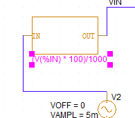
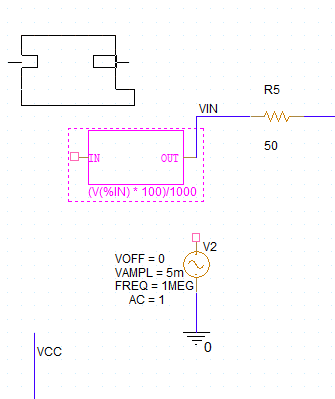
Step 9: Double-click the expression (V(%IN) * 100)/1000 to change the ABM expression.

Step 10: Enter V(%IN) + (RND-0.5)/500 for the value and click OK.

Running the Transient Simulation

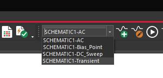
Step 11: Select SCHEMATIC1-Transient from the Active Simulation Profile drop-down menu at the top of the schematic.

Step 12: Select PSpice > Run from the menu.

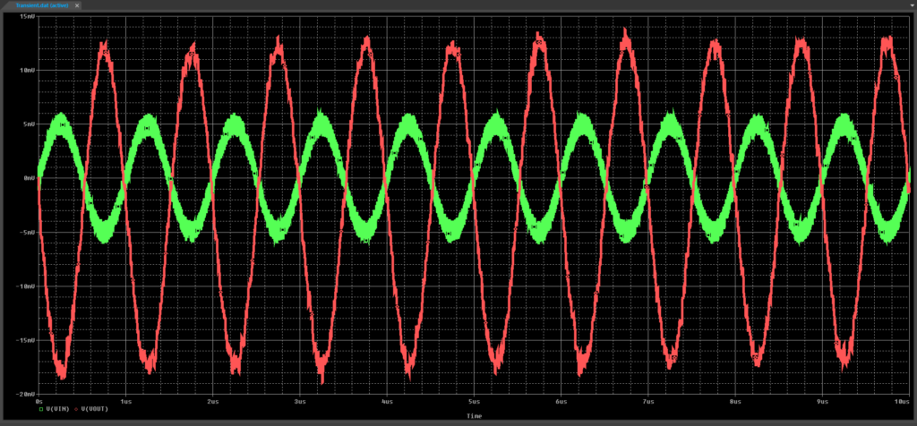
Step 13: View the simulation results. A noisier version of the RF amplifier waveform is shown.

Creating a Low Pass Filter ABM

Note: Analog behavioral models can be used to introduce mathematical expressions, such as an ideal low-pass filter.

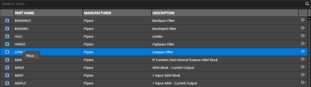
Step 14: Close the plot window. Back in the unified CIS tab, select the LOPASS ABM. Right-click and select Place.

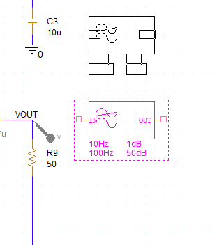
Step 15: Click to place the ABM in the circuit at the VOUT net. Right-click and select End Mode.

Step 16: Select Place > Wire from the menu, the Wire button from the toolbar, or press W on the keyboard.

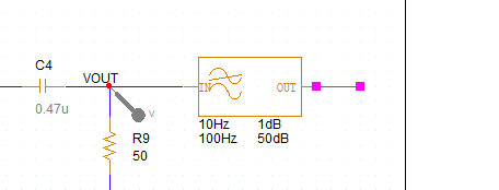
Step 17: Click to connect the ABM input to the VOUT net and add a short wire to the output. Press Escape on the keyboard when finished.

Step 18: Select Place > Net Alias from the menu, the Net Alias button from the toolbar, or press N on the keyboard.

Step 19: Enter VOUT_LPF as the alias and click OK.

Step 20: Click to place the alias on the ABM output. Right-click and select End Mode.

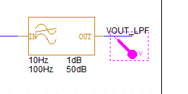
Step 21: Click and drag the marker on VOUT to place it on VOUT_LPF to analyze the LPF output.

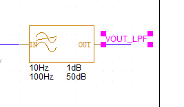
Step 22: Double-click the value of 10Hz to change the pass frequency.

Step 23: Enter a value of 3MEGHz and click OK.

Note: A value of 3MHz would be interpreted as 3 millihertz.

Step 24: Double-click the value of 100Hz to change the stop frequency.

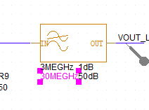
Step 25: Enter a value of 30MEGHz and click OK. The ABM filter has been configured.

Running the Transient Simulation

Step 26: Select PSpice > Run from the menu.

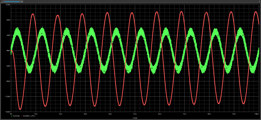
Step 27: View the simulation results. The input is still noisy but the output at VOUT_LPF is much cleaner.

Running the AC Sweep

Step 28: Close the plot window. Back in Capture, select the SCHEMATIC1-AC simulation from the Active Simulation Profile dropdown.

Step 29: Select PSpice > Run from the menu.

Step 30: The plot window opens to the original plot of V(VOUT). Double-click V(VOUT) in the legend of the top plot.

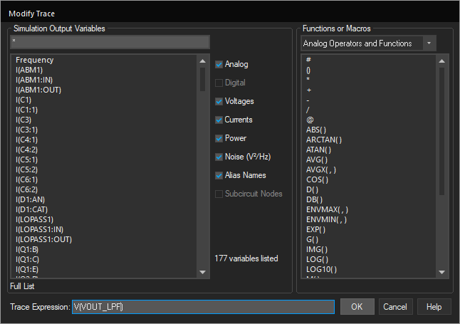
Step 31: Change the trace expression to V(VOUT_LPF). Click OK.

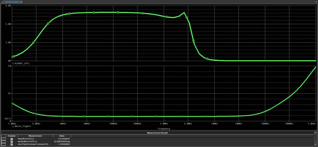
Step 32: View the results. The V(VOUT_LPF) plot now shows a strong cutoff past 3MHz.