While it is possible to get close to ideal component values with tight tolerances and precision manufacturing, truly ideal components only exist in simulation space. As a result, the analysis of a circuit in the real world may yield different measurements than that of a simulation and circuit operation may fall outside of the functional requirements. With PSpice Designer, analyze product yield and plot the output of a circuit across a range of component values within their tolerances with Monte Carlo analysis.
This quick how-to will provide step-by-step instructions on how to analyze product yield with Monte Carlo Analysis in PSpice Designer.
For step-by-step instructions on how to perform Monte Carlo analysis automatically with PSpice Designer Plus, view this how-to.
To follow along, download the provided files above the table of contents.
How-To Video
 Open in New Window
Creating a Parameter List
Step 1: Open the provided design in PSpice Designer.
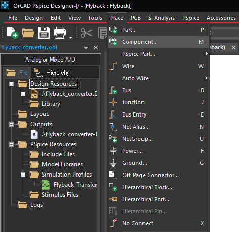
Step 2: Monte Carlo analysis works by varying component values within their tolerances, which can be defined in a parameter list. To place a parameter list, select Place > Component from the menu.
Step 3: The Component Explorer tab opens. From here, you can place components with PSpice models assigned as well as components from SamacSys, Ultra Librarian, and other sources.
Expand the PSpice category and select Simulator Command > Setup.
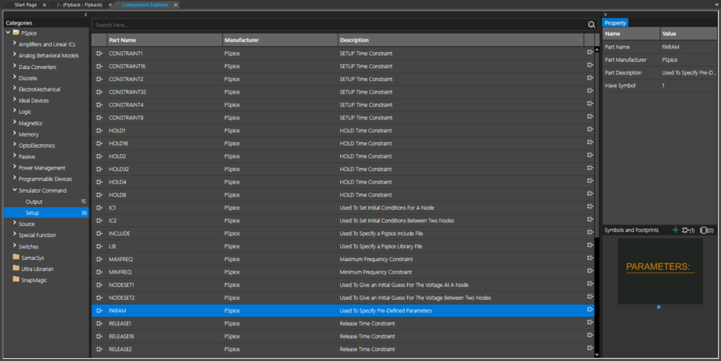
Step 4: Select PARAM from the part list and double-click to attach it to your cursor.
Note: This is a parameter list that can be used to define global parameters such as common tolerances.
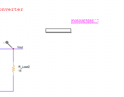
Step 5: Click to place the parameter list in the schematic, then right-click and select End Mode.
Defining Component Tolerances
Step 6: Common tolerances can be defined in the parameter list. To add parameters, double-click the list.
Step 7: The Property Editor tab opens. All properties for the selected object are defined in this window, as well as any global parameters for a PARAM list. Select New Property to add a new parameter.
Step 8: The Add New Property window opens. Enter CTOL for the property name and 0.10 for the value.
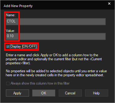
Step 9: Check Display [On/Off] to show the property on the parameter list object. Click OK.
Step 10: The Display Properties window opens. Select Both if Value Exists for the Display Format and click OK.
Step 11: Select New Property again.
Step 12: Enter LTOL for the property name and 0.20 for the value. Check Display [On/Off] and click OK.
Step 13: In the Display Properties window, select Both if Value Exists and click OK.
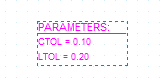
Step 14: Click Apply and close the Property Editor tab. The tolerance parameters are shown on the PCB canvas.
Assigning Component Tolerances
Step 15: With tolerance parameters defined, tolerances must be assigned to the relevant components as well. Double-click capacitor C4 to open the Property Editor tab.
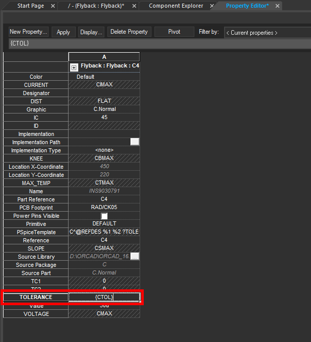
Step 16: The Property Editor tab for C4 is shown. Select the cell for Tolerance and enter {CTOL} to assign the CTOL parameter as the component tolerance.
Step 17: Click Apply and close the Property Editor tab.
Step 18: Hold CTRL on the keyboard and click inductors L1 and L2 to select them.
Step 19: Right-click one of the inductors and select Edit Properties to open the Property Editor tab for both inductors.
Step 20: Right-click the header cell for the Tolerance row and select Edit to define the tolerance for both inductors.
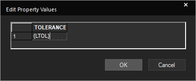
Step 21: The Edit Property Values window opens. Enter {LTOL} for the property and click OK.
Step 22: Select Apply and close the Property Editor tab.
Defining the Monte Carlo Sweep
Step 23: With tolerances assigned, a Monte Carlo sweep can be run. A simulation is already defined for this circuit. To edit the simulation, select PSpice > Edit Simulation Profile from the menu.
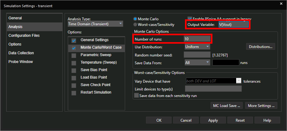
Step 24: The Simulation Settings window opens. Under Options, check Monte Carlo/Worst Case.
Step 25: Set the Number of Runs to 10 and the Output Variable to V(Vout). Leave the other settings as the defaults and click OK.
Running the Simulation
Step 26: To start the simulation, select PSpice > Run from the menu.
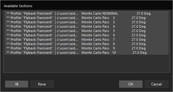
Step 27: The Available Sections window opens. Here you can configure which runs to display in the simulation plot. Select All to show all runs and click OK.
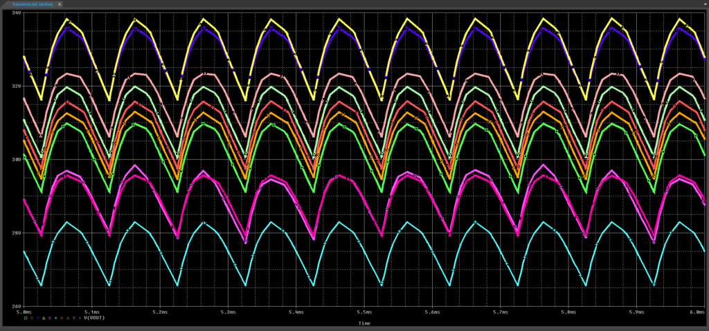
Step 28: View the simulation results. The green trace is the nominal trace plotted with ideal components. The other traces show several probable outputs of the circuit by randomizing the values of C4, L1, and L2 within their defined tolerances ranges. This gives an idea of possible real-world behavior.
Analyze Product Yield
Step 29: Performance analysis can be run to determine how much V(Vout) varies with each component value change. Select Trace > Performance Analysis from the menu to activate performance analysis.

Step 30: The Performance Analysis window opens. Select Wizard to open the Performance Analysis wizard.
Step 31: The Performance Analysis Wizard welcome screen opens. Click Next.
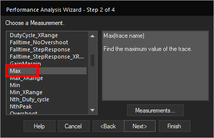
Step 32: The first step in the wizard is to define the measurement. Choose Max from the list and click Next.
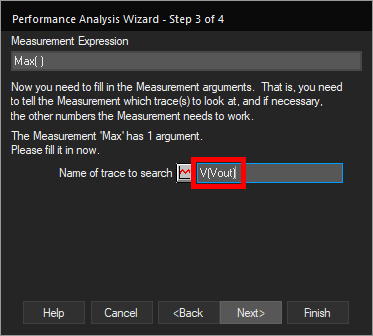
Step 33: Next, the measurement arguments must be defined. Enter V(Vout) as the name of the trace to search and click Next.
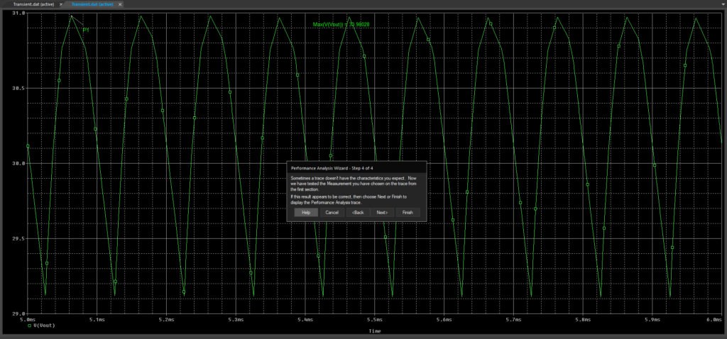
Step 34: A test trace is shown in the PSpice A/D window. To display the full performance analysis trace, select Finish.
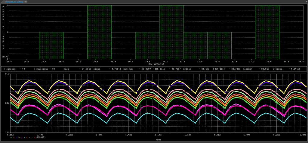
Step 35: View the results. A probability density graph is shown above the trace plot, indicating the most likely values of Max(V(Vout)).
Wrap Up & Next Steps
Quickly determine circuit behavior with component tolerances taken into account and analyze product yield with Monte Carlo Analysis in PSpice. Test out this feature and more with a free trial of OrCAD. Want to learn more about Monte Carlo Analysis and the other advanced analysis options in PSpice? View the Level 1 and Level 2 PSpice Advanced Analysis Workshops.

