Lesson 13: Non-Ideal Components

This walk-through will show how to define and add non-ideal components in PSpice to produce a more realistic simulation. After you complete this topic, you will be able to:

• Define and generate non-ideal capacitors
• Add tolerance parameters
• Run and compare the simulations

To follow along, continue with the design from the previous topic or use the provided materials.

If materials were not downloaded at the beginning of the walk-through, files for this lesson can be accessed through the materials tab above.

Saving the Simulation Results

Step 1: If you already closed the plot window, select PSpice > View Simulation Results from the menu to reopen it.

Step 2: Select File > Save As from the menu.

Step 3: Browse for a location to save the simulation DAT file. Name the file AC_Ideal.dat and click Save.

Step 4: Close the plot window.

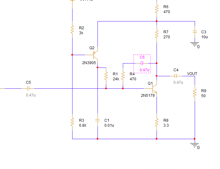
Creating Non-Ideal Capacitors

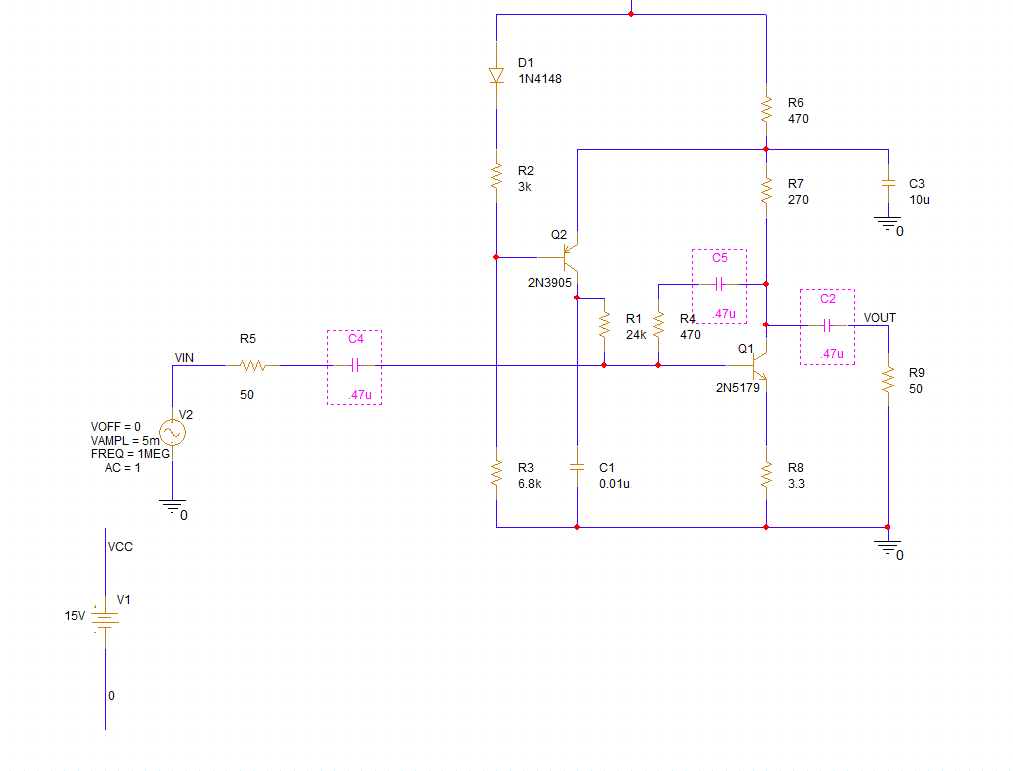
Step 5: Hold CTRL on the keyboard and select all capacitors with a value of 0.47u.

Step 6: Press Delete on the keyboard to delete the capacitors.

Step 7: If the Modeling Application is not open, select Place > PSpice Part > Modeling Application.

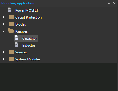
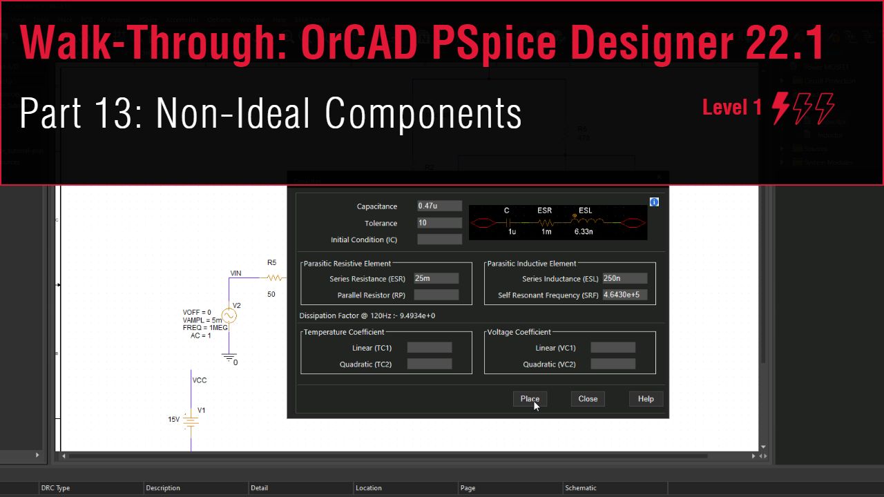
Step 8: Expand Passives and select Capacitor. The Capacitor window opens.

Note: Here you can define non-ideal parameters for a capacitor such as series resistance and tolerance.

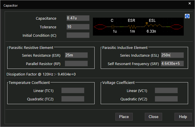
Step 9: Configure the following values:

• Capacitance: 0.47u
• Tolerance: 10
• Equivalent Series Resistance: 25m
• Equivalent Series Inductance: 250n

Note: When the equivalent series inductance (ESL) is defined, the Self Resonant Frequency field is automatically populated.

Step 10: Click Place.

Step 11: Click to place the capacitor in one of the empty spaces in the schematic.

Step 12: Select the capacitor and press CTRL-C on the keyboard.

Step 13: Press CTRL-V to paste and click to place the capacitor to fill the remaining empty spaces.

Running the Simulation

Step 14: Select PSpice > Run from the menu.

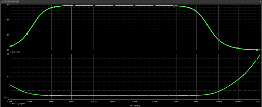
Step 15: View the results. A similar AC sweep is plotted, but the noise values are higher and the signal bandwidth is smaller.

Comparing the Simulations

Step 16: Select File > Open from the menu or the Open button from the toolbar.

Step 17: Browse to the location of AC_Ideal.dat and select it. Click Open.

Note: A tab labeled AC_Ideal.dat opens with a blank plot.

Step 18: Select Plot > Add Plot to Window from the menu.

Step 19: Select Trace > Add Trace.

Step 20: Select V(VOUT) from the Simulation Output Variables list. Click OK to add the trace to the upper plot.

Step 21: Select the bottom plot and select Trace > Add Trace again.

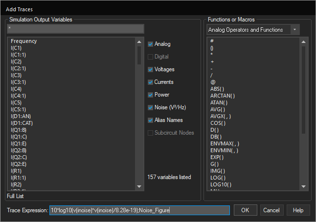
Step 22: Copy the expression 10*log10(v(inoise)*v(inoise)/8.28e-19);Noise_Figure and paste it into the Trace Expression field.

Step 23: Click OK to add the trace and close the window.

Step 24: Select View > Measurement Results from the menu.

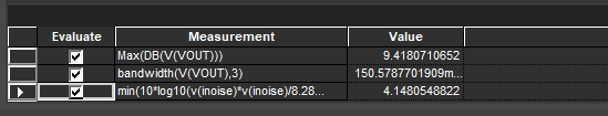
Step 25: Check Evaluate for all three measurements for AC_Ideal.

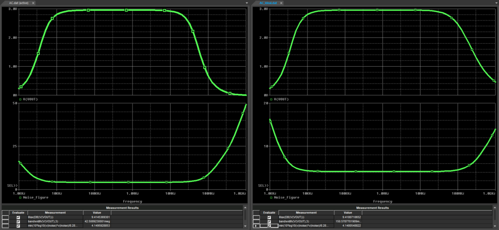
Step 26: Click and drag the AC_Ideal.dat tab to the right to set up a split screen configuration. Compare the waveforms and measurement results. The maximum V(VOUT) is similar between the two, but the bandwidth for the ideal plot is much wider.