Lesson 7: Transient Analysis

This walk-through will show to set up and run a transient analysis in OrCAD PSpice Designer 22.1. A transient analysis is a time-domain plot of the simulation parameters, equivalent to what would be seen on an oscilloscope if the circuit was tested in a lab. After you complete this topic, you will be able to:

• Configure and perform a transient analysis
• Create simulation models with the Modeling Application
• Add a secondary plot to the result window
• Use cursors in the plot window
• Add text and labels to a PSpice plot

To follow along, continue with the design from the previous topic or use the provided materials.

If materials were not downloaded at the beginning of the walk-through, files for this lesson can be accessed through the materials tab above.

Building an Emitter Follower Circuit

Note: For this example, we will modify the BJT circuit to create the Emitter Follower configuration.

Step 1: Select the wire between the emitter of Q1 and ground and press Delete on the keyboard.

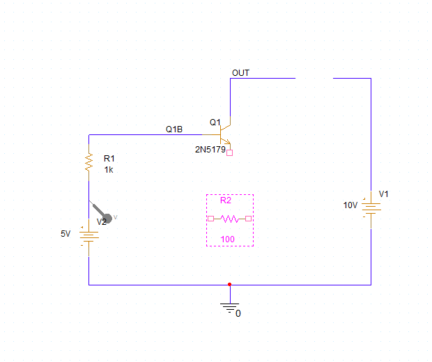
Step 2: Hold Alt on the keyboard and click and drag resistor R2 to move it between Q1 and ground.

Note: Holding Alt will prevent any wires connected to the component from moving as well.

Step 3: With R2 selected, press R on the keyboard to rotate it.

Step 4: Select Place > Wire from the menu, the Wire button from the toolbar, or press W on the keyboard.

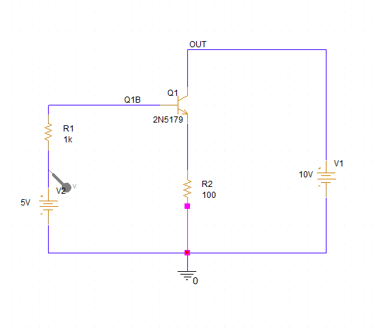
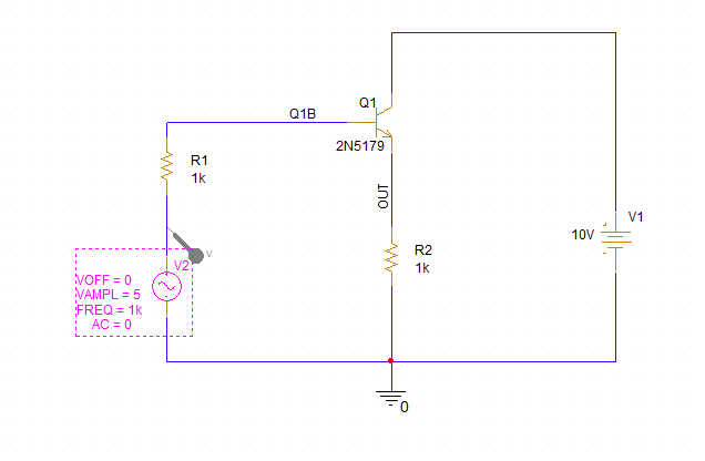
Step 5: Click to connect the wires broken by removing R2 and click to connect R2 to the emitter of Q1 and ground. Press Escape on the keyboard when finished.

Step 6: Double-click the value of R2. Change the value to 1k and click OK.

Step 7: Click and drag the net alias, OUT, to place it between the emitter of Q1 and R2.

Note: Click and drag R2 for more room as needed. Select a reference designator and press R on the keyboard to rotate the label.

Creating a Sine Source

Step 8: Select source V2 and press Delete on the keyboard.

Note: While the transient analysis will work with a DC input to the transistor, the results at OUT will be relatively constant.

Step 9: Select Place > PSpice Part > Modeling Application from the menu.

Note: The modeling application can be used to create custom models of non-ideal components and a wide variety of sources.

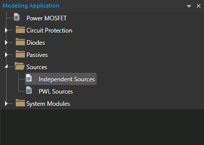
Step 10: The Modeling Application panel opens. Expand the Sources folder and select Independent Sources.

Step 11: Select the Sine tab.

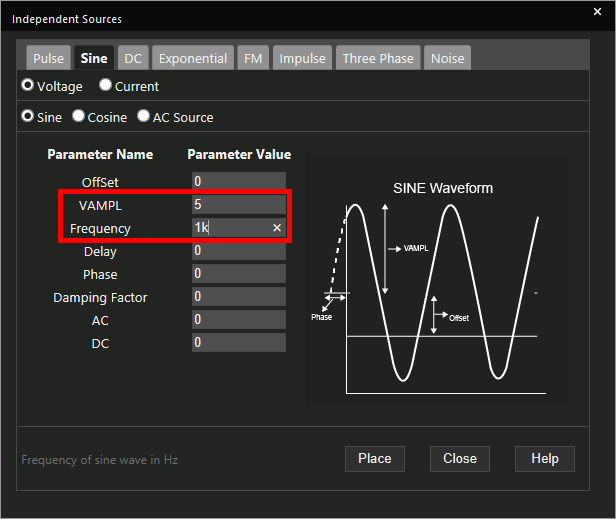
Step 12: Set the amplitude voltage (VAMPL) to 5 and the frequency to 1k.

Step 13: Click Place.

Step 14: Click to place the source where V2 was located.

Configuring a Transient Analysis

Step 15: Select PSpice > New Simulation Profile from the menu.

Step 16: Name the new simulation Transient and click Create.

Note: A transient simulation is a measurement of the circuit in the time domain. The results of the simulation are presented as if the circuit is being tested with an oscilloscope. This is the only type of simulation that can be performed on digital designs.

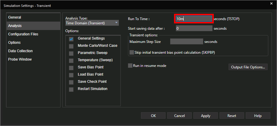
Step 17: The Simulation Settings window opens. Set the Run To Time to 10m.

Note: Set maximum step size to determine how many points are measured during the run time. Setting up a maximum step allows you to set a step size that is less than the default.

Step 18: Click OK to create the simulation profile.

Note: Probes have been removed from the circuit as each simulation profile requires its own set of probes.

Step 19: Select the Voltage/Level Marker button from the toolbar or PSpice > Markers > Voltage Level from the menu.

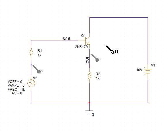
Step 20: Click to place probes on the net between V2 and R1 and the OUT net. Right-click and select End Mode.

Running the Simulation

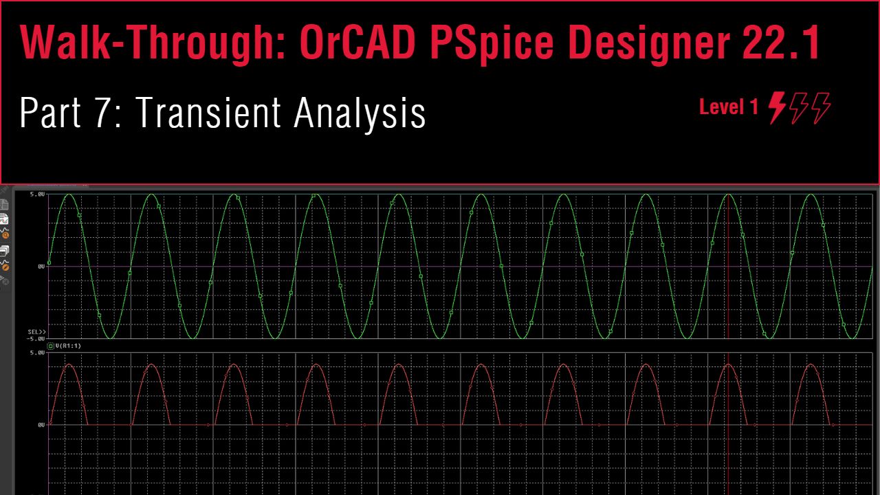
Step 21: Select PSpice > Run from the menu to run the simulation.

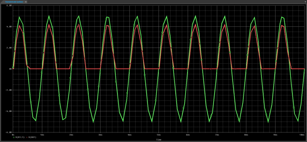
Step 22: View the simulation results.

Note: The waveforms results are not providing the level of detailed required. This can be seen in the waveform by the jagged and rough transitions for the trace, indicating that the maximum step size is too high.

Step 23: Select Simulation > Edit Profile from the menu or the Edit Simulation Settings button from the toolbar.

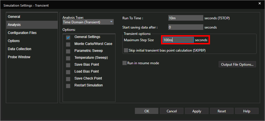
Step 24: Enter 100ns for the Maximum Step Size and click OK.

Step 25: Select Simulation > Run from the menu or the Run button from the toolbar.

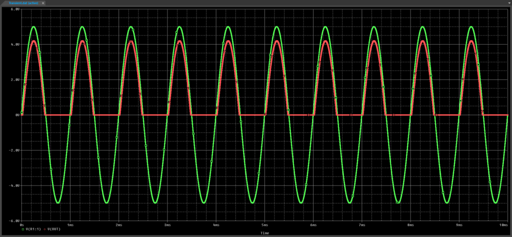
Step 26: View the results.

Note: The waveform has been smoothed.

Creating a Secondary Plot

Step 27: Select Plot > Add Plot to Window from the menu.

Note: A plot is created above the existing plot and automatically selected.

Step 28: Select V(R1:1) in the legend at the bottom of the first plot.

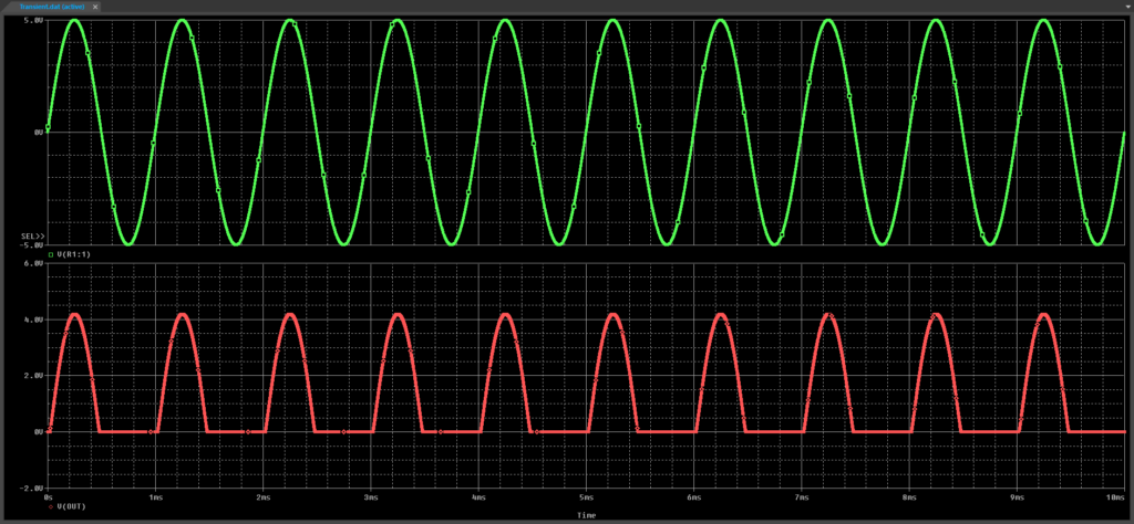
Step 29: Press CTRL-X on the keyboard to remove and copy the trace and CTRL-V to paste it to the new plot.

Activating and Using Cursors

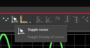
Step 30: Cursors can be used to make numerical measurements in the plot. Select the Toggle Cursor button from the toolbar to activate the cursor.

Note: This can also be activated by selecting Trace > Cursor > Display from the menu.

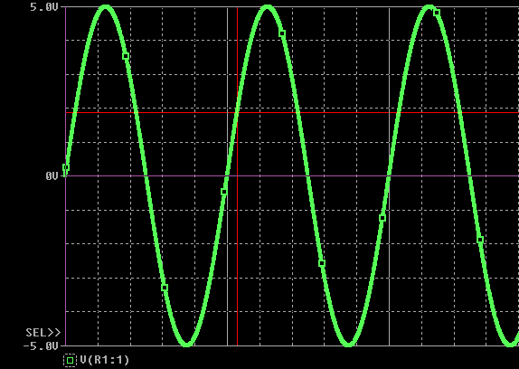
Step 31: Either click a location on the plot to view the corresponding measurements or click and drag in the plot to move the cursor crosshairs.

Note: The active trace is indicated with a dotted box around the corresponding trace symbol. Select the symbol next to a trace name to change the active trace.

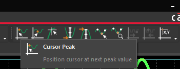
Step 32: Select the Cursor Peak button in the toolbar to move the cursor to the next relative maximum.

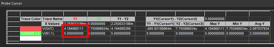
Note: The numeric values are listed for both traces in the Probe Cursor panel.

Step 33: Select Cursor Trough in the toolbar to move the cursor to the next relative minimum.

Step 34: Select Cursor Max in the toolbar to move the cursor to the absolute maximum.

Note: Since this is a periodic wave, the calculated absolute maximum and minimum could be any one of the peaks or troughs.

Adding Plot Labels

Step 35: Select the label for V(OUT) on the lower plot and select the plot itself.

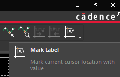
Step 36: Select the Mark Label button from the toolbar. A label with the current cursor coordinates is placed on the plot.

Step 37: Select the Text Label button from the toolbar.

Step 38: Enter the text Max(V(VOUT)) and click OK.

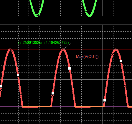
Step 39: Click to place the label near the cursor coordinates.